Regional Economic Descriptive Analysis
1. Description
The Regional Economic Descriptive Analysis module in LUMENS evaluates the economic dynamics of a region, providing insights into key indicators such as GDP, sectoral contributions, employment, and income distribution. By analyzing these trends, the module helps stakeholders understand the economic drivers of land use and resource allocation. This information is crucial for policymakers facing real-world challenges, such as balancing economic growth with sustainable land use, improving livelihoods, and optimizing land-use policies.
2. Usage
2.1 Workflow
This module processes input economic data such as GDP, contribution per sector and employment, along with spatial data for the region of interest. Users can define key parameters such as unit, location, and time period. Once the data and parameters are set, the module processes the input data, analyzing the regional economy based on indicators such as GDP growth, sectoral contribution to the economy, and employment trends over the selected time period. The module outputs a comprehensive set of results, including descriptive statistics, graphs, and visualizations that showcase the economic trends within the region. This includes metrics such as the dominance of certain sectors, changes in employment rates, and overall land-based economic performance.
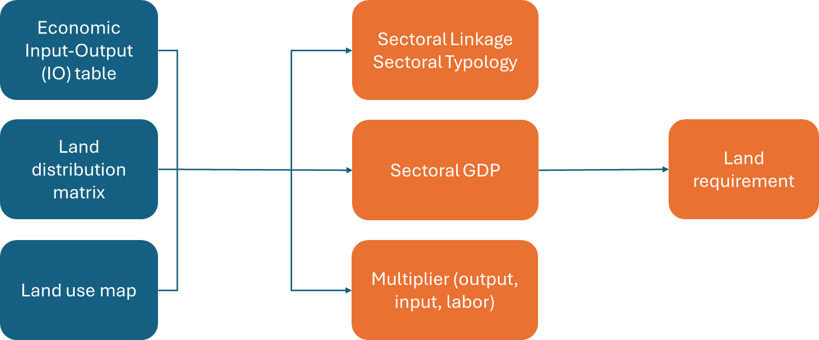
2.2 Step-by-step instructions
Step 1: Uploading Economic and Land Use Data
In this step, you’ll upload four data sets required for analysis.
Upload Input Output Table
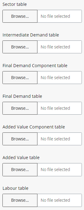
- Click the “Browse” Button in the economic sections.
- Select your Table (CSV format), the IO table should be divided into seven different tables: sector, intermediate demand, final demand component, final demand, added value component, added value and labor table.
- When the data is successfully uploaded, it will appear as follows.
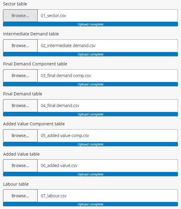
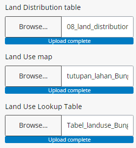
Upload Input Land Use Data
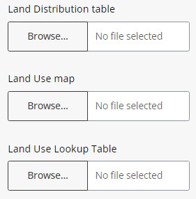
- Click the “Browse” Button in the land sections.
- Select your Table (CSV and TIFF format), the land use data are: land distribution table, land use map and land use look up table.
- When the data is successfully uploaded, it will appear as follows.
Step 2: Setting Analysis Parameters
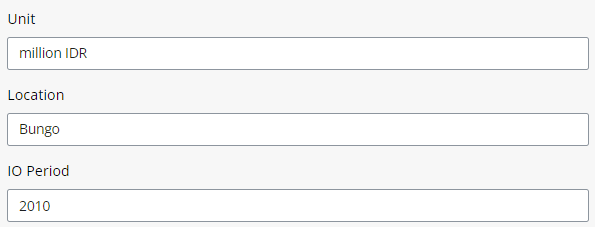
These parameters include the analysis unit, location, and Input-Output period.
Analysis Unit
- Enter the unit, it defines the currency in which the economic results are expressed, such as “million IDR.”
- Fill in location refers to the name of the district or region.
- Enter the IO period to indicate the year in which the Input-Output table was produced.
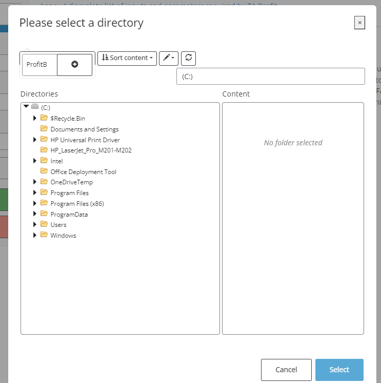
- Select Output Directory where results will be saved, Click ‘+’ to save and Select.
Step 3: Running the Analysis
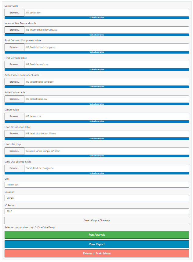
Once all data is uploaded and parameters are set, run the analysis. Results will appear in the “Results” tab.
2.3 Tips
For large datasets, the analysis may take some time to complete.
3. Data Requirements
3.1 Input Data & Parameters
| No | Data Name | Type | Format | Projection Requirements | Description |
|---|---|---|---|---|---|
| 1. | Sector | Categorical | CSV | N/A | Economic sectors such as agriculture, industry, or services. |
| 2. | Intermediate Demand | Numerical | CSV | N/A | The purchase of a commodity by domestic industries as an input to production, excluding capital investment. |
| 3. | Final Demand Component | Numerical | CSV | N/A | The total demand for economic output in all sectors across the region. |
| 4. | Final Demand | Numerical | CSV | N/A | The total demand for economic output in all sectors across the region. |
| 5. | Added Value Component | Numerical | CSV | N/A | Sum of unit profit (revenue minus intermediate consumption). |
| 6. | Added Value | Numerical | CSV | N/A | Sum of unit profit (revenue minus intermediate consumption). |
| 7. | Labour | Numerical | CSV | N/A | Number of workers employed per sector. |
| 8. | Land Distribution | Numerical | CSV | N/A | Represent allocation of land among different sectors. |
| 9. | Land Use Map | Categorical raster | GeoTIFF | UTM | A land use map detailing spatial land classifications by economic sector, showing how land is utilized across the region. |
| 10. | Land Use Lookup | Text | CSV | N/A | A lookup table that links land use codes from spatial data sets to specific economic sectors or land use types for reference and analysis purposes. |
Include rows for ALL required input data and parameters.
3.2 Example Datasets
Example data sets can be accessed in link.

3.3 Data Acquisition
Provide guidance on finding suitable data, linking to common sources if applicable. Example: - Land cover maps can often be obtained from link to data source. - For creating your own land cover maps from satellite imagery, consider using software such as link to software.
4. Outputs
4.1 Output Files
| File Name | Type | Description |
|---|---|---|
land_use_change_map_[SUFFIX].tif |
Raster | Map depicting changes in land use between the specified time periods. |
transition_matrix_[SUFFIX].csv |
CSV | Table showing the area of land that transitioned between each land use category. |
report_[SUFFIX].html |
HTML | A report summarizing the analysis results with visualizations and tables. |
| … | … | … |
Include rows for ALL output files, including the report.
4.2 Report Interpretation
This section provides users with guidance on interpreting the content of the generated report, drawing insights from sectoral linkages, GDP analysis, multiplier effects, and land requirements. Understanding these results can aid in policy and decision making.
1. Analysis of Sectoral Linkages
Sectoral linkage consists of Direct Backward Linkage (DBL) and Direct Forward Linkage (DFL) represents connection between sector in a regional economy.
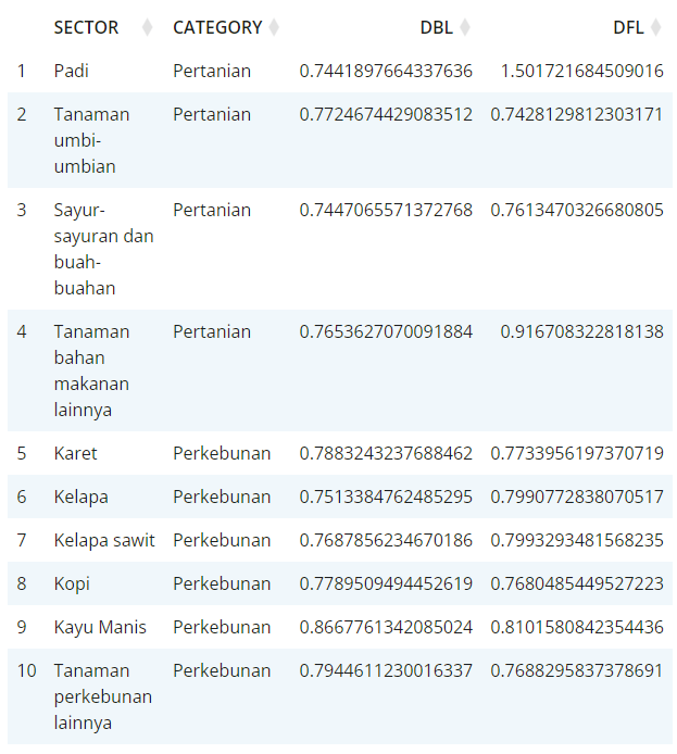
Direct Backward Linkage (DBL): This indicates how much demand a sector creates for inputs from other sectors. If a sector shows a strong backward linkage, it suggests that it relies heavily on other industries for resources and services.
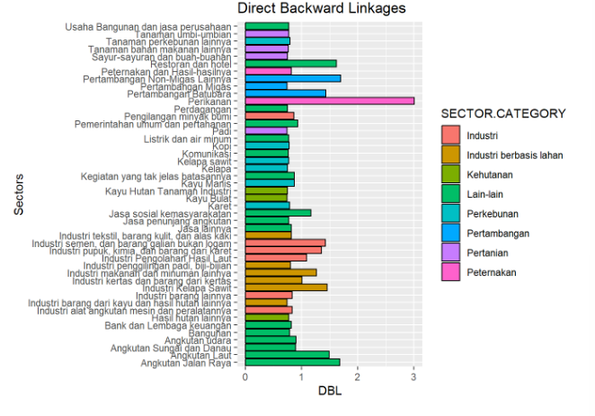
A high backward linkage in fisheries (perikanan) means that expanding this sector will boost demand for inputs from upstream industries, such as raw materials and intermediate goods. Policymakers might focus on strengthening supply chains for these industries to support the growth.
If agriculture (pertanian) shows weak backward linkages, interventions could aim to improve integration with suppliers (e.g., fertilizers, machinery) to enhance sectoral efficiency.
Direct Forward Linkage (DFL): This measures how much output from a sector is used as an input by other sectors. A high forward linkage implies that many industries depend on this sector’s output.
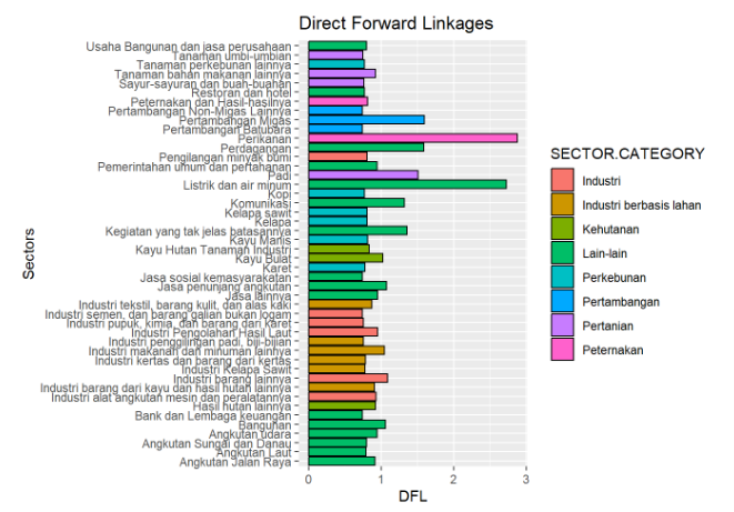
If the service (jasa/lain-lain) sector exhibits strong forward linkages, improvements in energy production can positively impact other industries like manufacturing, transport, and services.
Policymakers could prioritize investments in communication (komunikasi) infrastructure to reduce costs and stimulate industrial productivity, based on strong forward linkage results.
Sectoral Typology: This categorizes sectors based on their linkages and growth potential. Sectors can be classified as key sectors, dependent sectors, or independent sectors.
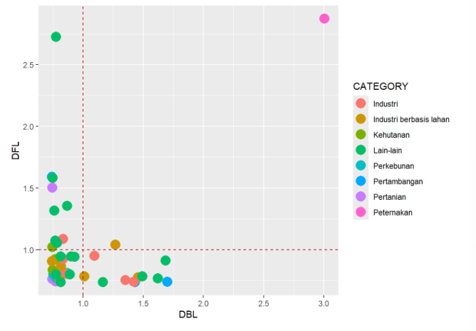
Key sectors exhibit both strong forward and backward linkages, meaning they play a crucial role in the region’s economy, in this graph is livestock (peternakan). Development efforts could prioritize these sectors to maximize overall economic impact, it would be a priority for both investment and policy support because of its ripple effects across multiple industries.
Graph Interpretation: The forward and backward linkage graph helps visualize these relationships, highlighting which sectors drive demand for inputs and supply outputs critical for the economy.
2. Analysis of GDP
The GDP table presents data for each sector’s contribution to the region’s GDP, showing trends over time. This can reveal whether certain sectors are growing or shrinking in economic significance.
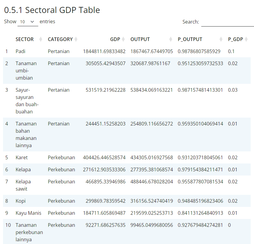
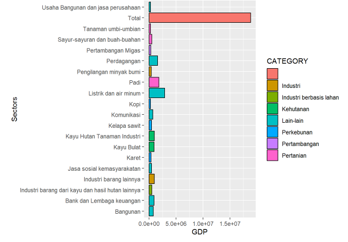
The accompanying graph visually represents GDP growth by sector, making it easier to spot trends such as emerging industries or declining traditional sectors. In this graph, electricity and water (listrik dan air) is the leading GDP sector, followed by trade (perdagangan). This graphs showed that Bungo’s economic dominated by service or secondary industry.
3. Analysis of Multiplier
Output Multiplier: This shows how much additional output is generated for each unit of output in a sector. A high output multiplier indicates that a sector has strong spillover effects on the wider economy.
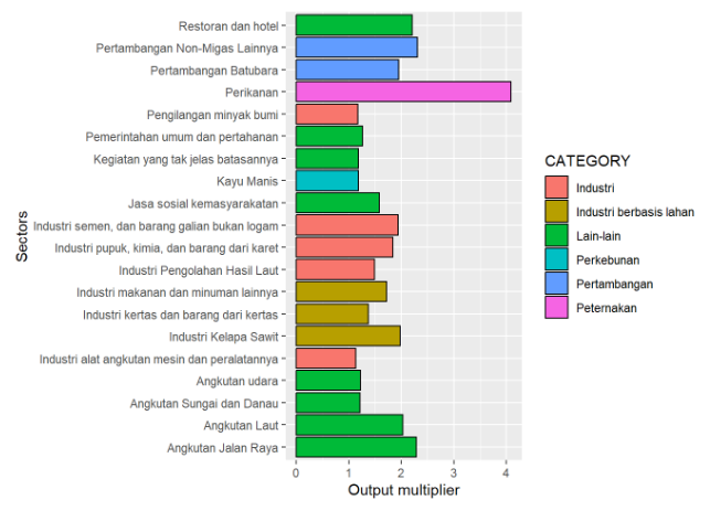
If the fisheries (perikanan) sector has a high output multiplier, it means that expanding construction activities will drive significant additional production in related sectors like fish feed (pakan) and transportation.
Policymakers might focus on promoting fisheries projects as part of a stimulus strategy, leveraging its strong multiplier effect to boost overall economic growth.
Input Multiplier: This reflects how much additional input a sector demands from others. Sectors with high input multipliers create substantial demand for upstream products.
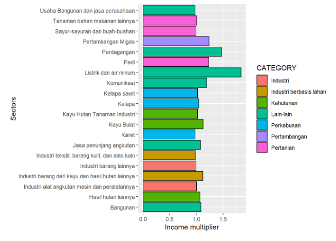
If the electricity and water (listrik dan air minum) sector has a high input multiplier, enhancing its productivity can stimulate demand in raw materials and intermediate goods sectors.
Promoting domestic supply chains for rice (padi) can reduce dependency on imports, strengthen local industries, and generate employment.
Labour Multiplier: This represents the number of jobs generated for each unit of output in a sector. A high labor multiplier indicates that the sector is labor-intensive and can create employment opportunities.
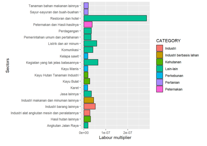
If restaurant and hotels exhibits a high labor multiplier, supporting this sector can lead to significant job creation, especially in tourism areas.
Policymakers might design tourism development programs focused on ecotourism to balance between economic and environmental health.
4. Land Requirement Table and Coefficient
Land Requirement: This table outlines the amount of land required by each sector based on production levels and sectoral needs. It quantifies how much land is used or will be needed to sustain economic activities.
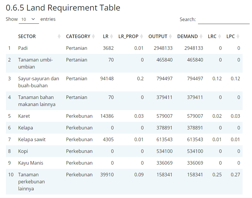
A high land requirement for agriculture (pertanian) might indicate that increased agricultural output is land-intensive, potentially leading to land scarcity or environmental degradation. Sustainable land use practices should be considered in such cases.
If service sectors show lower land requirements but high output, this could suggest that economic development could be shifted towards more land-efficient service to preserve natural resources.
Land Use Coefficient: This coefficient represents the efficiency of land use by each sector. A higher coefficient means that a sector uses land more efficiently relative to its output.
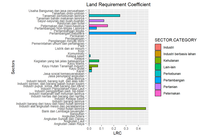
Sectors with low land use coefficients (e.g., agriculture) may require modernization or shifts to more efficient practices to increase productivity while minimizing land consumption.
If forestry shows a high land requirement coefficient, policies might focus on reforestation or sustainable forestry management to enhance land use efficiency while supporting environmental goals.
5. Theoretical Background
5.1 Model Description
The Regional Economy Descriptive Analysis Module is designed to assess and interpret the economic structure and relationships within a region. The model relies on input-output (I-O) analysis, which captures interdependencies between sectors in an economy, while also incorporating spatial data for land use analysis. This allows for a comprehensive understanding of how different sectors interact, their contribution to the region’s GDP, and their impact on land use and employment.
5.2 Key Assumptions
Key assumptions used in this module are as follows:
- It is assumed that the inter-sectoral relationships in the economy, as captured by the input-output (I-O) tables, remain stable throughout the analysis period. Changes in technology, trade, or consumption patterns are not considered.
- Land use changes occur linearly over the analysis period.
5.3 Limitations
The module limitations and potential sources of error/uncertainty are as follows:
- This module does not account for gradual land use changes or changes that occur within a single land use category.
- Accuracy is limited by the quality and resolution of the input land cover maps.
References
@article{jensen1988study, title={The study of regional economic structure using input–output tables}, author={Jensen, Rodney C and West, Guy R and Hewingst, GJD}, journal={Regional Studies}, volume={22}, number={3}, pages={209–220}, year={1988}, publisher={Taylor \& Francis} }
